前些天發現了一個巨牛的人工智能學習網站，通俗易懂，風趣幽默，忍不住分享一下給大家。點擊跳轉到網站。

集成學習

---

集成學習（ensemble learning）博采眾家之長，通過構建并結合多個學習器來完成學習任務。“三個臭皮匠頂個諸葛亮”，一個學習器（分類器、回歸器）效果可能并不好，通過結合若干學習器取得更好的效果，進一步提高精度等。

工作原理是?成多個學習器，每個學習器獨?地學習并作出預測。這些預測最后結合成組合預測，因此優于任何?個單分類的做出預測。不難理解，如果3個學習器的預測結果是2正1負，若基于簡單投票，則組合預測結果就是正，故也稱為基于委員會的學習。

對于弱學習器（效果略優于隨機猜測的學習器）來說，集成效果尤為明顯。已證明，隨著個體分類器數量的增加，集成的錯誤率將指數級下降，最終區域零。

但是如果生成的個體學習器的差異太小，得出的結果基本一致，那么集成學習后也不會有什么改善提高。也就是說，個體學習器應好而不同，既有一定準確性，又有一定多樣性。

為了解決這個問題，一種方法是使用不同的算法，如分別用支持向量機、決策樹、樸素貝葉斯、KNN等生成個體學習器。但更主流的是另一種方法：使用同種算法。

那新的問題是，怎么保證同種算法訓練出的學習器有差異性呢？自然只能從數據下手。根據依賴性，可分為Bagging和Bosting兩種方法。

Bagging

---

Bagging（Bootstrap Aggregating）生成個體學習器時，學習器之間沒有任何依賴，也就是并行的生成個體學習器，主要解決過擬合。

Bagging主要關注降低方差。通過使用自助采樣法，即通過有放回的抽樣方式，生成n個新的數據集，并用這些數據集分別訓練n個個體學習器，最后使用多數投票或取均值等結合策略生成集成器。

• 自助采樣法

自助采樣法（Bootstrap sampling）是對原始數據有放回的均勻采樣，放回意味著可能重復抽到同一樣本，也可能從來抽不到一些樣本（約占36.8%），這些樣本可用作測試集來對泛化性能進行評估。

• 結合策略

結合策略包括平均法、投票法和學習法。

對數值輸出型可采用平均法。設$T$個個體學習器$h_1,h_2,...h_T$，用$h_i(x)$表示$h_i$在示例$x$上的輸出。
簡單平均法：$$H(x)=\frac{1}{T}\sum _{i=1}^T{h}_i(x)$$
加權平均法：$$H(x)=\sum _{i=1}^T{w}_i{h}_i(x)$$

對分類任務可采用投票法。學習器$h_i$從類別$c_1,c_2,...,c_N$中預測類別，用$h_i^j(x)$表示$h_i$在類別$c_j$上的輸出。
絕對多數投票法：超過半數則預測為該類別，否則拒絕。$$H(x)=\{\begin{array}{l}{c}_j,if{\sum }_{i=1}^T{h}_i^j(x)>0.5{\sum }_{k=1}^N{\sum }_{i=1}^T{h}_i^k(x)\\ reject,otherwise\end{array}$$
相對多數投票法：$$H(x)=c_{argma{x}_j{\sum }_{i=1}^T{h}_i^j(x)}$$
加權投票法：$$H(x)=c_{argma{x}_j{\sum }_{i=1}^T{w}_i{h}_i^j(x)}$$

學習法通過另一個學習器來進行結合，如Stacking算法先從初始數據集訓練出初級學習器，然后用初級學習器的輸出作為次級學習器的輸入，從而對初級學習器進行結合。簡單說就是套娃。

隨機森林

---

隨機森林（Random Forest，RF）是Bagging的一個擴展變體，顧名思義是對決策樹的集成。

決策樹是在選擇劃分屬性時，是在當前數據集所有特征屬性集合中選擇一個最優屬性。而在隨機森林中，對基決策樹的每個結點，先從該結點的屬性集合中隨機選擇一個包含$k$個屬性的子集，然后再在該子集中選擇最優屬性。

對原始數據集每次隨機的選擇$k$個屬性，構成$n$個新數據集并訓練基決策樹，然后采用投票法等結合策略進行集成。而$k$的取值，一般推薦$k=lo{g}_{2}d$，$d$為屬性個數。

可以使用sklearn庫中的RandomForestClassifier()函數創建隨機森林分類模型，RandomForestRegressor()函數創建隨機森林回歸模型。
默認用基尼指數作為劃分依據，包括一些剪枝參數等，可查文檔不再贅述。

分類應用示例：

import matplotlib.pyplot as plt
import numpy as np
import pandas as pd
from matplotlib.colors import ListedColormap
from sklearn.datasets import make_blobs
from sklearn.ensemble import RandomForestClassifier
from sklearn.model_selection import train_test_split
from sklearn.metrics import classification_report
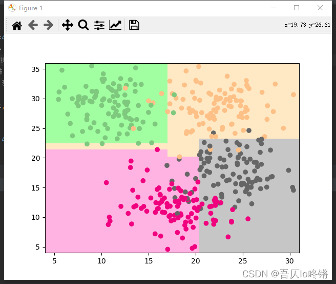
import seaborn as snsdef plot_boundary(model, axis):  # 畫邊界x0, x1 = np.meshgrid(np.linspace(axis[0], axis[1], int((axis[1] - axis[0]) * 100)).reshape(-1, 1),np.linspace(axis[2], axis[3], int((axis[3] - axis[2]) * 100)).reshape(-1, 1),)X_new = np.c_[x0.ravel(), x1.ravel()]y_predict = model.predict(X_new)zz = y_predict.reshape(x0.shape)custom_cmap = ListedColormap(['#A1FFA1', '#FFE9C5', '#FFB3E2', '#C6C6C6'])plt.contourf(x0, x1, zz, cmap=custom_cmap)# 創建數據：400個樣本，2個特征，4個類別，方差3
X, y = make_blobs(400, 2, centers=4, cluster_std=3, center_box=(10, 30), random_state=20221026)
x_train, x_test, y_train, y_test = train_test_split(X, y)  # 劃分訓練集測試集
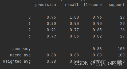
rf = RandomForestClassifier()  # 隨機森林
rf.fit(x_train, y_train)  # 訓練
y_pred = rf.predict(x_test)  # 測試
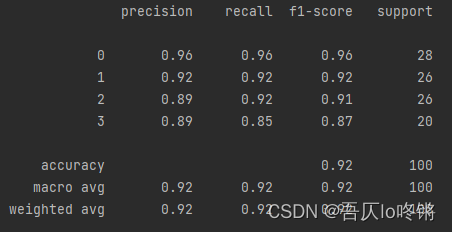
# 評估
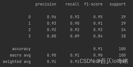
print(classification_report(y_test, y_pred))
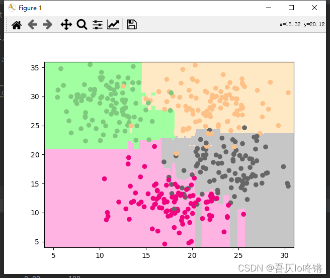
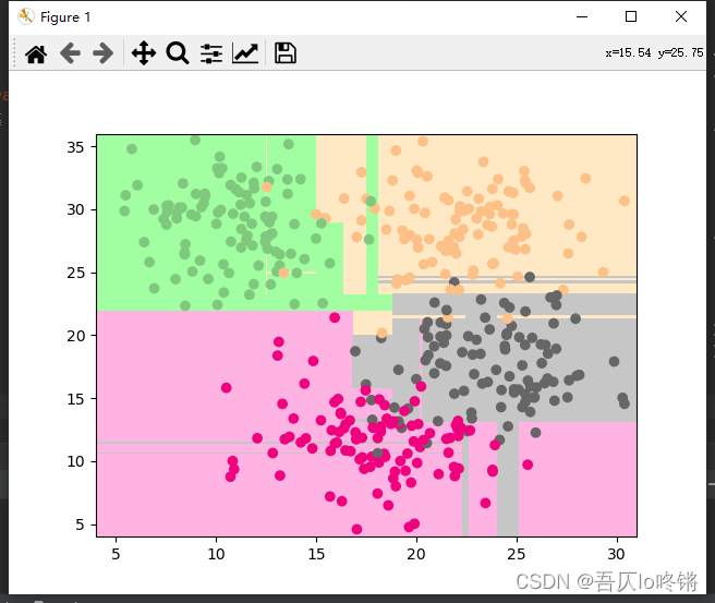
# 可視化
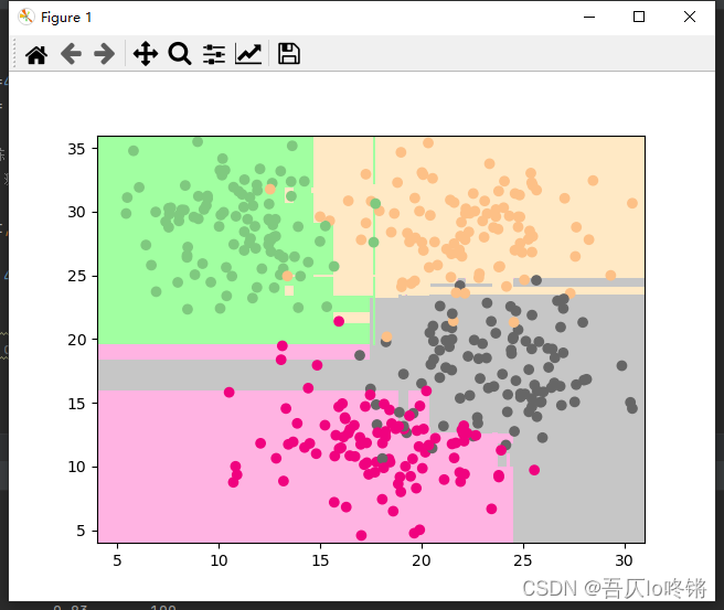
plot_boundary(rf, axis=[4, 31, 4, 36])  # 邊界
plt.scatter(X[:, 0], X[:, 1], c=y, cmap='Accent')  # 數據點
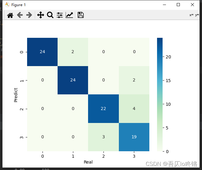
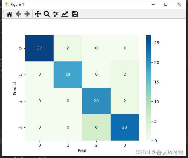
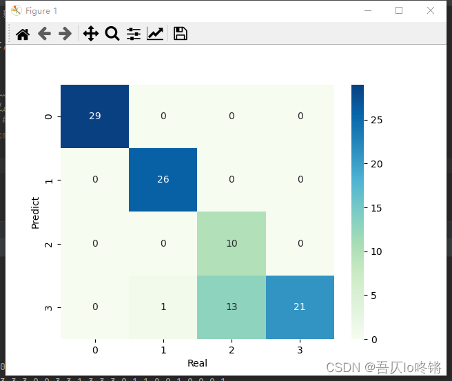
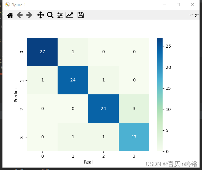
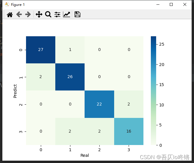
#cm = pd.crosstab(y_pred, y_test)  # 混淆矩陣
#sns.heatmap(data=cm, annot=True, cmap='GnBu', fmt='d')
#plt.xlabel('Real')
#plt.ylabel('Predict')
plt.show()

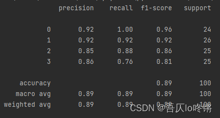
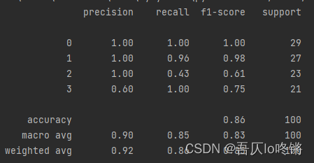
隨機森林的結果是普遍優于決策樹的，RF還有一些其他變體，這里不再深入。

為方便比較（后同），給出決策樹結果：

Bosting

---

Bosting生成個體學習器時，學習器之間存在強依賴，后一個學習器是對前一個學習器的優化，也就是串行（序列化）的生成個體學習器，主要解決欠擬合

Bosting主要關注增加模型復雜度來降低偏差。先從初始訓練集訓練出一個基學習器，再根據基學習器的表現對訓練樣本分布進行調整，使先前學習做錯的訓練樣本得到更多關注，即放大做錯樣本的權重，重復進行，直至基學習器個數達到指定值，最終將這些基學習器進行加權結合。

與Bagging自助采樣不同，Boosting使用全部訓練樣本，根據前一個學習器的結果調整數據的權重，然后串行的生成下一個學習器，最后根據結合策略進行集成。

核心問題就是權重的調整和結合策略，主要有3種算法：Adaboost、GBDT、XGBoost。

Adaboost

---

Adaboost（Adaptive Boosting）基本分類器組成的加法模型，損失函數為指數損失函數，適用于分類任務。主要思想是對上一個基學習器的結果，提高分類錯誤樣本的權重，降低分類正確樣本的權重，然后通過加權后各基模型進行投票表決進行集成。

省去億點點推導，多分類主要步驟是：

1. 初始化樣本權重$w_0=\frac{1}{m}$，m是訓練樣本數。

2. 訓練學習器，計算誤差$e_t$。$$e_t=w_0\sum _{i=1}^m(y\_tru{e}_i!=y\_pre{d}_i)$$

3. 更新學習器權重：R表示分類數量。$${\alpha }_t=learnin{g}_{r}ate?(ln\frac{1?e^t}{e^t}+ln(R?1))$$

4. 更新樣本權重：$Z_t$是歸一化因子，表示所有樣本權重的和。$$w_t=\frac{w_{t?1}?exp({\alpha }_t?(y\_true!=y\_pred))}{Z_t}$$

5. 循環步驟2-4，訓練T個學習器，加權投票得到集成器：$$H(x)=sign(\sum _{t=1}^T{\alpha }_t{h}_t(x))$$

可以使用sklearn中的AdaBoostClassifier()函數創建Adaboost分類模型，AdaBoostRegressor()函數創建Adaboost回歸模型，默認基學習器是決策樹。
參數n_estimators是基學習器個數，默認50，過大易過擬合。learning_rate學習率默認1，過大易錯過最優值，過小收斂慢。

分類應用示例：

import matplotlib.pyplot as plt
import numpy as np
import pandas as pd
from matplotlib.colors import ListedColormap
from sklearn.datasets import make_blobs
from sklearn.ensemble import AdaBoostClassifier
from sklearn.model_selection import train_test_split
from sklearn.metrics import classification_report
import seaborn as snsdef plot_boundary(model, axis):  # 畫邊界x0, x1 = np.meshgrid(np.linspace(axis[0], axis[1], int((axis[1] - axis[0]) * 100)).reshape(-1, 1),np.linspace(axis[2], axis[3], int((axis[3] - axis[2]) * 100)).reshape(-1, 1),)X_new = np.c_[x0.ravel(), x1.ravel()]y_predict = model.predict(X_new)zz = y_predict.reshape(x0.shape)custom_cmap = ListedColormap(['#A1FFA1', '#FFE9C5', '#FFB3E2', '#C6C6C6'])plt.contourf(x0, x1, zz, cmap=custom_cmap)# 創建數據：400個樣本，2個特征，4個類別，方差3
X, y = make_blobs(400, 2, centers=4, cluster_std=3, center_box=(10, 30), random_state=20221026)
x_train, x_test, y_train, y_test = train_test_split(X, y)  # 劃分訓練集測試集
model = AdaBoostClassifier()  # AdaBoost
model.fit(x_train, y_train)  # 訓練
y_pred = model.predict(x_test)  # 測試
# 評估
print(classification_report(y_test, y_pred))
# 可視化
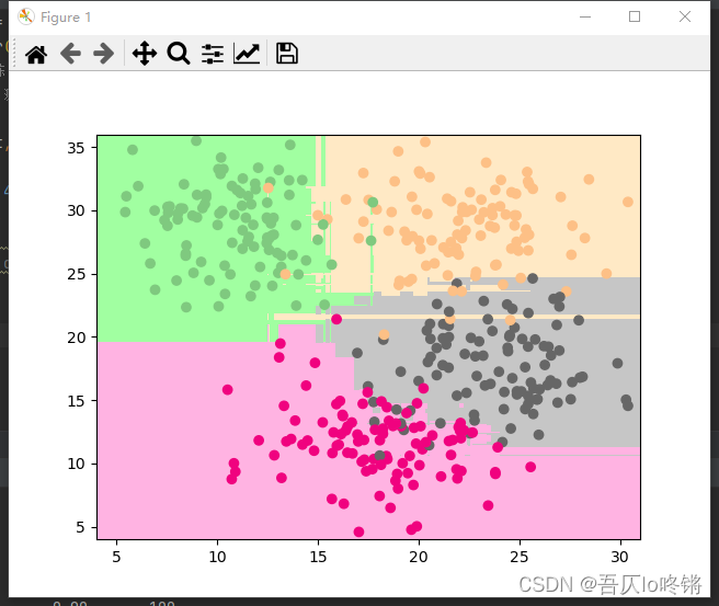
plot_boundary(model, axis=[4, 31, 4, 36])  # 邊界
plt.scatter(X[:, 0], X[:, 1], c=y, cmap='Accent')  # 數據點
#cm = pd.crosstab(y_pred, y_test)  # 混淆矩陣
#sns.heatmap(data=cm, annot=True, cmap='GnBu', fmt='d')
#plt.xlabel('Real')
#plt.ylabel('Predict')
plt.show()

（插播反爬信息 ）博主CSDN地址：https://wzlodq.blog.csdn.net/

GBDT

---

GBDT（Gradient Boosting Decision Tree）梯度提升決策樹，即梯度下降 + Boosting + 決策樹，是以決策樹為基學習器，以樣本殘差代替分類錯誤率作為模型提升的標準。

思想步驟基本與AdaBoost一致，只是將錯誤率用殘差來計算，即真實值與預測值的差距，而最小殘差的計算需要帶入梯度公式，置偏導為0，求解梯度下降最大的負方向，即如名梯度提升決策樹。也就是說損失函數同線性回歸中最小二乘。

可以使用sklearn中的GradientBoostingClassifier()函數創建GBDT分類模型，GradientBoostingRegressor()函數創建GBDT回歸模型，默認基學習器是決策樹。

分類應用示例：

import matplotlib.pyplot as plt
import numpy as np
import pandas as pd
from matplotlib.colors import ListedColormap
from sklearn.datasets import make_blobs
from sklearn.ensemble import GradientBoostingClassifier
from sklearn.model_selection import train_test_split
from sklearn.metrics import classification_report
import seaborn as snsdef plot_boundary(model, axis):  # 畫邊界x0, x1 = np.meshgrid(np.linspace(axis[0], axis[1], int((axis[1] - axis[0]) * 100)).reshape(-1, 1),np.linspace(axis[2], axis[3], int((axis[3] - axis[2]) * 100)).reshape(-1, 1),)X_new = np.c_[x0.ravel(), x1.ravel()]y_predict = model.predict(X_new)zz = y_predict.reshape(x0.shape)custom_cmap = ListedColormap(['#A1FFA1', '#FFE9C5', '#FFB3E2', '#C6C6C6'])plt.contourf(x0, x1, zz, cmap=custom_cmap)# 創建數據：400個樣本，2個特征，4個類別，方差3
X, y = make_blobs(400, 2, centers=4, cluster_std=3, center_box=(10, 30), random_state=20221026)
x_train, x_test, y_train, y_test = train_test_split(X, y)  # 劃分訓練集測試集
model = GradientBoostingClassifier()  #梯度提升決策樹
model.fit(x_train, y_train)  # 訓練
y_pred = model.predict(x_test)  # 測試
# 評估
print(classification_report(y_test, y_pred))
# 可視化
plot_boundary(model, axis=[4, 31, 4, 36])  # 邊界
plt.scatter(X[:, 0], X[:, 1], c=y, cmap='Accent')  # 數據點
#cm = pd.crosstab(y_pred, y_test)  # 混淆矩陣
#sns.heatmap(data=cm, annot=True, cmap='GnBu', fmt='d')
#plt.xlabel('Real')
#plt.ylabel('Predict')
plt.show()

XGBoost

---

XGBoost（eXtreme Gradient Boosting）算法本質上也是梯度提升決策樹算法（GBDT），但其速度和效率較前者更高，是進一步優化改良，可理解為二階泰勒展開+ boosting + 決策樹 + 正則化。

對目標函數進行優化，用泰勒展開來近似目標，泰勒展開式含二階導數利于梯度下降更快更準，可以不知到損失函數的顯示表達，通過數據帶入就可進行結點分裂計算。

同時添加正則項，預防過擬合，提高模型泛化能力。

sklearn庫中并沒有封裝較新的XGBoost算法，可以安裝開源的xgboost庫：

pip install xgboost

使用xgboost庫中XGBClassifier()函數創建XGBoost分類模型，XGBRegressor()函數創建XGBoost回歸模型。

分類應用示例：

import matplotlib.pyplot as plt
import numpy as np
import pandas as pd
from matplotlib.colors import ListedColormap
from sklearn.datasets import make_blobs
from xgboost import XGBClassifier
from sklearn.model_selection import train_test_split
from sklearn.metrics import classification_report
import seaborn as snsdef plot_boundary(model, axis):  # 畫邊界x0, x1 = np.meshgrid(np.linspace(axis[0], axis[1], int((axis[1] - axis[0]) * 100)).reshape(-1, 1),np.linspace(axis[2], axis[3], int((axis[3] - axis[2]) * 100)).reshape(-1, 1),)X_new = np.c_[x0.ravel(), x1.ravel()]y_predict = model.predict(X_new)zz = y_predict.reshape(x0.shape)custom_cmap = ListedColormap(['#A1FFA1', '#FFE9C5', '#FFB3E2', '#C6C6C6'])plt.contourf(x0, x1, zz, cmap=custom_cmap)# 創建數據：400個樣本，2個特征，4個類別，方差3
X, y = make_blobs(400, 2, centers=4, cluster_std=3, center_box=(10, 30), random_state=20221026)
x_train, x_test, y_train, y_test = train_test_split(X, y)  # 劃分訓練集測試集
model = XGBClassifier()  #XGBoost
model.fit(x_train, y_train)  # 訓練
y_pred = model.predict(x_test)  # 測試
# 評估
print(classification_report(y_test, y_pred))
# 可視化
plot_boundary(model, axis=[4, 31, 4, 36])  # 邊界
plt.scatter(X[:, 0], X[:, 1], c=y, cmap='Accent')  # 數據點
#cm = pd.crosstab(y_pred, y_test)  # 混淆矩陣
#sns.heatmap(data=cm, annot=True, cmap='GnBu', fmt='d')
#plt.xlabel('Real')
#plt.ylabel('Predict')
plt.show()

原創不易，請勿轉載（本不富裕的訪問量雪上加霜 ）
博主首頁：https://wzlodq.blog.csdn.net/
來都來了，不評論兩句嗎👀
如果文章對你有幫助，記得一鍵三連?