多核CPU已经成为现代计算机体系结构发展的标准,不仅可以在超级计算机设备中找到,也可以在我们的家用台式机和笔记本电脑中找到;就连苹果(Apple)的iPhone 5S在2013年也配备了1.3 Ghz双核处理器。
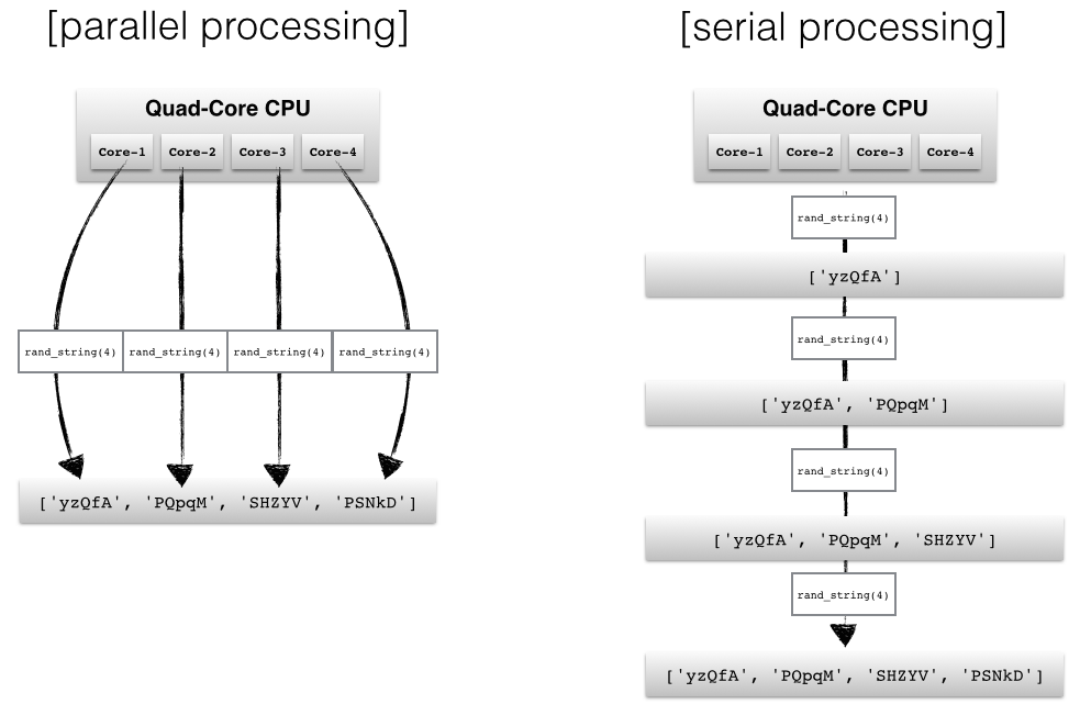
网络模块怎么打、然而,默认的Python解释器在设计时考虑到了简单性,并具有线程安全机制,即所谓的GIL(全局解释器锁)。为了防止线程之间的冲突,它一次只执行一条语句(所谓的串行处理,或单线程)。
在这篇 Python 多进程模块的介绍中,我们将看到如何生成多个子进程来避免 GIL 的一些缺点。
wx模块,根据应用程序的不同,并行编程中的两种常见方法是分别通过线程或多个进程运行代码。如果我们将任务提交给不同的线程,这些作业可以被描绘为单个进程的子任务,并且这些线程通常可以访问相同的内存区域(即共享内存)。这种方法在不正确同步的情况下很容易导致冲突,例如,如果进程在同一时间写相同的内存位置。 一种更安全的方法(尽管由于不同进程之间的通信开销而带来额外的开销)是将多个进程提交到完全独立的内存位置(即分布式内存):每个进程将完全独立地运行。
在这里,我们将看看 Python 的多进程模块,以及我们如何使用它来提交可以彼此独立运行的多个进程,以充分利用我们的 CPU 内核。
Python 标准库中的multiprocessing模块有很多强大的功能。如果您想了解所有的技巧和细节,我建议您使用官方文档作为入口点。
在接下来的部分中,我想简要概述不同的方法,以展示multiprocessing模块如何用于并行编程。
最基本的方法可能是使用multiprocessing模块中的 Process 类。 在这里,我们将使用一个简单的队列函数来并行生成四个随机字符串。
import multiprocessing as mp
import random
import stringrandom.seed(123)# Define an output queue
output = mp.Queue()# define a example function
def rand_string(length, output):""" Generates a random string of numbers, lower- and uppercase chars. """rand_str = ''.join(random.choice(string.ascii_lowercase+ string.ascii_uppercase+ string.digits)for i in range(length))output.put(rand_str)# Setup a list of processes that we want to run
processes = [mp.Process(target=rand_string, args=(5, output)) for x in range(4)]# Run processes
for p in processes:p.start()# Exit the completed processes
for p in processes:p.join()# Get process results from the output queue
results = [output.get() for p in processes]print(results)
# ['BJWNs', 'GOK0H', '7CTRJ', 'THDF3']
获得结果的顺序不一定要与进程的顺序(在进程列表中)相匹配。由于我们最终使用 .get() 方法从队列中按顺序检索结果,因此进程完成的顺序决定了我们结果的顺序。 例如,如果第二个进程在第一个进程之前完成,则结果列表中字符串的顺序也可能是 ['PQpqM', 'yzQfA', 'SHZYV', 'PSNkD'] 而不是 ['yzQfA' , 'PQpqM', 'SHZYV', 'PSNkD']。
如果我们的应用程序要求我们按特定顺序检索结果,一种可能性是引用进程的 ._identity 属性。在本例中,我们也可以简单地使用range对象中的值作为位置参数。修改后的代码为:
import multiprocessing as mp
import random
import stringrandom.seed(123)
# Define an output queue
output = mp.Queue()# define a example function
def rand_string(length, pos, output):""" Generates a random string of numbers, lower- and uppercase chars. """rand_str = ''.join(random.choice(string.ascii_lowercase+ string.ascii_uppercase+ string.digits)for i in range(length))output.put((pos, rand_str))# Setup a list of processes that we want to run
processes = [mp.Process(target=rand_string, args=(5, x, output)) for x in range(4)]# Run processes
for p in processes:p.start()# Exit the completed processes
for p in processes:p.join()# Get process results from the output queue
results = [output.get() for p in processes]print(results)
# [(0, 'h5hoV'), (1, 'fvdmN'), (2, 'rxGX4'), (3, '8hDJj')]
并且检索到的结果将是元组,例如,[(0, 'KAQo6'), (1, '5lUya'), (2, 'nj6Q0'), (3, 'QQvLr')] 或 [(1, '5lUya'), (3, 'QQvLr'), (0, 'KAQo6'), (2, 'nj6Q0')]。
为了确保我们按顺序检索结果,我们可以简单地对结果进行排序,并可选择去掉 position 参数:
results.sort()
results = [r[1] for r in results]
print(results)
# ['h5hoV', 'fvdmN', 'rxGX4', '8hDJj']
维护有序结果列表的一种更简单的方法是使用 Pool.apply 和 Pool.map 函数,我们将在下一节中讨论。
Pool 类为简单的并行处理任务提供了另一种更方便的方法。
有四种方法特别有趣:
Pool.applyPool.mapPool.apply_asyncPool.map_asyncPool.apply 和 Pool.map 方法基本上等同于 Python 的内置 apply 和 map 函数。
在我们讨论 Pool 方法的async变体之前,让我们看一个使用 Pool.apply 和 Pool.map 的简单示例。在这里,我们将进程数设置为 4,这意味着 Pool 类将只允许 4 个进程同时运行。
def cube(x):return x**3
pool = mp.Pool(processes=4)
results = [pool.apply(cube, args=(x,)) for x in range(1,7)]
print(results)
# [1, 8, 27, 64, 125, 216]
pool = mp.Pool(processes=4)
results = pool.map(cube, range(1,7))
print(results)
# [1, 8, 27, 64, 125, 216]
Pool.map和Pool.apply将锁定主程序,直到所有进程完成,如果我们希望为特定的应用程序以特定的顺序获得结果,这是非常有用的。
相反,async变量将立即提交所有过程,并在它们完成后立即检索结果。另一个区别是,我们需要在apply_async()调用之后使用get方法,以便获得已完成进程的返回值。
pool = mp.Pool(processes=4)
results = [pool.apply_async(cube, args=(x,)) for x in range(1,7)]
output = [p.get() for p in results]
print(output)
# [1, 8, 27, 64, 125, 216]
在下面的方法中,我想对串行与多进程处理方法进行简单比较,其中我将使用稍微复杂的函数。
在这里,我定义了一个函数,使用Parzen-window技术对概率密度函数执行核密度估计。我不想详细介绍这种技术的理论,因为我们最感兴趣的是如何使用多进程处理来提高性能。
import numpy as npdef parzen_estimation(x_samples, point_x, h):"""Implementation of a hypercube kernel for Parzen-window estimation.Keyword arguments:x_sample:training sample, 'd x 1'-dimensional numpy arrayx: point x for density estimation, 'd x 1'-dimensional numpy arrayh: window widthReturns the predicted pdf as float."""k_n = 0for row in x_samples:x_i = (point_x - row[:,np.newaxis]) / (h)for row in x_i:if np.abs(row) > (1/2):breakelse: # "completion-else"*k_n += 1return (k_n / len(x_samples)) / (h**point_x.shape[1])
简单地说,这个函数的功能是:计算一个已定义区域(所谓的窗口)中的点数,然后将其中的点数除以总点数,从而估计一个点在某个区域中的概率。
下面是一个简单的例子,我们的窗口由一个以原点为中心的超立方体表示,我们希望根据超立方体估计一个点位于图中心的概率。
from mpl_toolkits.mplot3d import Axes3D
import matplotlib.pyplot as plt
import numpy as np
from itertools import product, combinations
fig = plt.figure(figsize=(7,7))
ax = fig.gca(projection='3d')
ax.set_aspect("equal")# Plot Points# samples within the cube
X_inside = np.array([[0,0,0],[0.2,0.2,0.2],[0.1, -0.1, -0.3]])X_outside = np.array([[-1.2,0.3,-0.3],[0.8,-0.82,-0.9],[1, 0.6, -0.7],[0.8,0.7,0.2],[0.7,-0.8,-0.45],[-0.3, 0.6, 0.9],[0.7,-0.6,-0.8]])for row in X_inside:ax.scatter(row[0], row[1], row[2], color="r", s=50, marker='^')for row in X_outside:    ax.scatter(row[0], row[1], row[2], color="k", s=50)# Plot Cube
h = [-0.5, 0.5]
for s, e in combinations(np.array(list(product(h,h,h))), 2):if np.sum(np.abs(s-e)) == h[1]-h[0]:ax.plot3D(*zip(s,e), color="g")ax.set_xlim(-1.5, 1.5)
ax.set_ylim(-1.5, 1.5)
ax.set_zlim(-1.5, 1.5)plt.show()
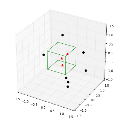
point_x = np.array([[0],[0],[0]])
X_all = np.vstack((X_inside,X_outside))print('p(x) =', parzen_estimation(X_all, point_x, h=1))
# p(x) = 0.3
在下面的部分中,我们将从二元高斯分布创建一个随机数据集,其中均值向量以原点为中心,单位矩阵作为协方差矩阵。
import numpy as npnp.random.seed(123)# Generate random 2D-patterns
mu_vec = np.array([0,0])
cov_mat = np.array([[1,0],[0,1]])
x_2Dgauss = np.random.multivariate_normal(mu_vec, cov_mat, 10000)
如下所示,分布中心点的预期概率约为 0.15915。 我们的目标是使用 Parzen-window 方法根据我们上面创建的样本数据集来预测这个密度。
为了通过Parzen-window技术做出好的预测,除了其他事情之外,选择一个合适的窗口是至关重要的。在这里,我们将使用多进程来预测使用不同窗宽的二元高斯分布中心的密度。
from scipy.stats import multivariate_normal
var = multivariate_normal(mean=[0,0], cov=[[1,0],[0,1]])
print('actual probability density:', var.pdf([0,0]))
# actual probability density: 0.159154943092
下面,我们将为串行和多进程方法建立基准测试函数,并将其传递给我们的timeit基准测试函数。
我们将使用Pool.apply_async函数来利用同时启动进程的优势:在这里,我们不关心计算不同窗口宽度的结果的顺序,我们只需要将每个结果与输入窗口宽度关联。
因此,我们对parzen_density_estimate函数做了一点小小的调整,返回一个包含两个值的元组:窗宽和估计密度,这将允许我们稍后对结果列表进行排序。
def parzen_estimation(x_samples, point_x, h):k_n = 0for row in x_samples:x_i = (point_x - row[:,np.newaxis]) / (h)for row in x_i:if np.abs(row) > (1/2):breakelse: # "completion-else"*k_n += 1return (h, (k_n / len(x_samples)) / (h**point_x.shape[1]))
def serial(samples, x, widths):return [parzen_estimation(samples, x, w) for w in widths]def multiprocess(processes, samples, x, widths):pool = mp.Pool(processes=processes)results = [pool.apply_async(parzen_estimation, args=(samples, x, w)) for w in widths]results = [p.get() for p in results]results.sort() # to sort the results by input window widthreturn results
只是想知道结果会是什么样子(即,不同窗口宽度的预测密度):
widths = np.arange(0.1, 1.3, 0.1)
point_x = np.array([[0],[0]])
results = []results = multiprocess(4, x_2Dgauss, point_x, widths)for r in results:print('h = %s, p(x) = %s' %(r[0], r[1]))# h = 0.1, p(x) = 0.016
# h = 0.2, p(x) = 0.0305
# h = 0.3, p(x) = 0.045
# h = 0.4, p(x) = 0.06175
# h = 0.5, p(x) = 0.078
# h = 0.6, p(x) = 0.0911666666667
# h = 0.7, p(x) = 0.106
# h = 0.8, p(x) = 0.117375
# h = 0.9, p(x) = 0.132666666667
# h = 1.0, p(x) = 0.1445
# h = 1.1, p(x) = 0.157090909091
# h = 1.2, p(x) = 0.1685
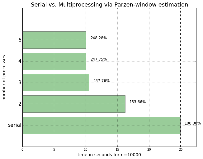
根据结果,我们可以说最佳窗口宽度是 h=1.1,因为估计结果接近实际结果 ~0.15915。
因此,对于基准测试,让我们在 1.0 到 1.2 的范围内创建 100 个均匀间隔的窗口宽度。
widths = np.linspace(1.0, 1.2, 100)import timeitmu_vec = np.array([0,0])
cov_mat = np.array([[1,0],[0,1]])
n = 10000x_2Dgauss = np.random.multivariate_normal(mu_vec, cov_mat, n)benchmarks = []benchmarks.append(timeit.Timer('serial(x_2Dgauss, point_x, widths)','from __main__ import serial, x_2Dgauss, point_x, widths').timeit(number=1))benchmarks.append(timeit.Timer('multiprocess(2, x_2Dgauss, point_x, widths)','from __main__ import multiprocess, x_2Dgauss, point_x, widths').timeit(number=1))benchmarks.append(timeit.Timer('multiprocess(3, x_2Dgauss, point_x, widths)','from __main__ import multiprocess, x_2Dgauss, point_x, widths').timeit(number=1))benchmarks.append(timeit.Timer('multiprocess(4, x_2Dgauss, point_x, widths)','from __main__ import multiprocess, x_2Dgauss, point_x, widths').timeit(number=1))benchmarks.append(timeit.Timer('multiprocess(6, x_2Dgauss, point_x, widths)','from __main__ import multiprocess, x_2Dgauss, point_x, widths').timeit(number=1))
准备绘制结果
import platform
from matplotlib import pyplot as plt
import numpy as npdef print_sysinfo():print('\nPython version :', platform.python_version())print('compiler :', platform.python_compiler())print('\nsystem :', platform.system())print('release :', platform.release())print('machine :', platform.machine())print('processor :', platform.processor())print('CPU count :', mp.cpu_count())print('interpreter:', platform.architecture()[0])print('\n\n')def plot_results():bar_labels = ['serial', '2', '3', '4', '6']fig = plt.figure(figsize=(10,8))# plot barsy_pos = np.arange(len(benchmarks))plt.yticks(y_pos, bar_labels, fontsize=16)bars = plt.barh(y_pos, benchmarks,align='center', alpha=0.4, color='g')# annotation and labelsfor ba,be in zip(bars, benchmarks):plt.text(ba.get_width() + 2, ba.get_y() + ba.get_height()/2,'{0:.2%}'.format(benchmarks[0]/be),ha='center', va='bottom', fontsize=12)plt.xlabel('time in seconds for n=%s' %n, fontsize=14)plt.ylabel('number of processes', fontsize=14)t = plt.title('Serial vs. Multiprocessing via Parzen-window estimation', fontsize=18)plt.ylim([-1,len(benchmarks)+0.5])plt.xlim([0,max(benchmarks)*1.1])plt.vlines(benchmarks[0], -1, len(benchmarks)+0.5, linestyles='dashed')plt.grid()plt.show()plot_results()
print_sysinfo()
Python version  : 3.4.1
compiler        : GCC 4.2.1 (Apple Inc. build 5577)system     : Darwin
release    : 13.2.0
machine    : x86_64
processor  : i386
CPU count  : 4
interpreter: 64bit
我们可以看到,如果我们并行提交它们,我们可以加快 Parzen-window函数的密度估计。但是,在我的特定机器上,提交 6 个并行 6 个进程并不会带来进一步的性能提升,这对于 4 核 CPU 来说是有意义的。 我们还注意到,当我们并行使用 3 个而不是仅 2 个进程时,性能显着提高。然而,当我们分别移动到 4 个并行进程时,性能提升并不显着。
这可以归因于在这种情况下,CPU 仅由 4 个内核组成,并且系统进程(例如操作系统)也在后台运行。因此,第四核根本没有足够的容量来进一步大幅提高第四进程的性能。而且我们还必须记住,每个额外的进程都会带来额外的进程间通信开销。
此外,只有当我们的任务是计算密集型时,并行处理带来的改进才有意义,其中大部分任务都花在 CPU 上,而不是 I/O 绑定任务,即处理来自磁盘的数据的任务。
https://sebastianraschka.com/Articles/2014_multiprocessing.html
版权声明:本站所有资料均为网友推荐收集整理而来,仅供学习和研究交流使用。

工作时间:8:00-18:00
客服电话
电子邮件
admin@qq.com
扫码二维码
获取最新动态


![[笔记]c++Windows平台代码规范](/upload/rand_pic/2-745.jpg)